2  Optimization

Optimization can mean different things. Mathematically speaking, it is possible to write and optimization problem in the form of:

\[ \min_{x \in \mathbb{R}^n} f_{i}(\mathbf{x}), \quad (i=1, 2, \dots, M)\] \[\textrm{subject to} \quad \phi_{j}(\mathbf{x}) = 0, \quad (j=1, 2, \dots, J)\] \[\quad \psi_{k}(\mathbf{x}) <= 0, \quad \quad (k=1, 2, \dots, K)\]

\(f_{i}(\mathbf{x})\), \(\phi_{j}(\mathbf{x})\) and \(\psi_{k}(\mathbf{x})\) are functions of the vector

\[\mathbf{x} = (x_{1}, x_{2}, \dots, x_{n})^T\]

where the components \(x_{i}\) of \(\mathbf{x}\) are called decision variables and they can be real continuous, discrete or a mixture of both.

The functions \(f_{i}(\mathbf{x}), (i=1, 2, \dots, M)\) are called the objective functions, and in the case of \(M=1\) there is only one objective. The space spanned by the decision variables is called the search space \(\mathbb{R}^n\), while the space formed by the objective function values is called the solution space. The objective function can be linear or nonlinear.

The equalities \(\phi_{j}(\mathbf{x})\) and inequalities \(\psi_{k}(\mathbf{x})\) are called constraints. The simplest case of the constraints is where \(x_{i}\) is \(x_{i, \min} \leq x_{i} \leq x_{i, \max}\), which is called bounds.

If the functions \(f_{i}(\mathbf{x})\), \(\phi_{j}(\mathbf{x})\) and \(\psi_{k}(\mathbf{x})\) are all linear, then we are in presence of a linear programming problem. For linear programming problems, a significant progress was the development of the simplex method in 1947 by George B. Dantzig.

A special class of optimization is where there is no contraint at all and the only task is to find the minimum or maximum of a single objective function \(f_{i}(\mathbf{x})\).

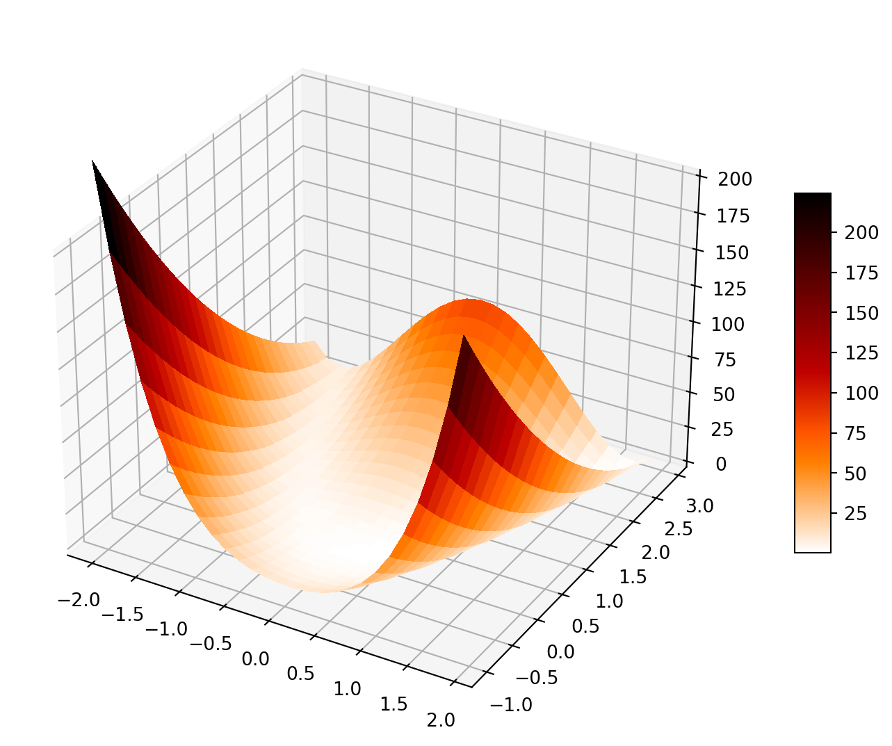
For example, imagine that you want to find the minimum of the Rosenbrock banana function:

\[f(x, y) = (1 - x)^2 + 100 \times (y - x^2)^2\]

Code

import numpy as np
import matplotlib.pyplot as plt
from matplotlib import cm
from matplotlib.ticker import LinearLocator, FormatStrFormatter
from mpl_toolkits.mplot3d import Axes3D

b = 10
f = lambda x,y: (1-x)**2 + b*(y-x**2)**2

# Initialize figure 
figRos = plt.figure(figsize=(12, 7))
axRos = figRos.add_subplot(projection='3d')

# Evaluate function
X = np.arange(-2, 2, 0.15)
Y = np.arange(-1, 3, 0.15)
X, Y = np.meshgrid(X, Y)
Z = f(X,Y)

# Plot the surface
surf = axRos.plot_surface(X, Y, Z, cmap=cm.gist_heat_r,
                       linewidth=0, antialiased=False)
axRos.set_zlim(0, 200)
figRos.colorbar(surf, shrink=0.5, aspect=10)
plt.show()

In order to find its minimum, we can set its partial derivatives to zero:

\[\frac{\partial f}{\partial x}=2(1-x) - 400(y-x^2) x = 0\] \[\frac{\partial f}{\partial y}=200(y-x^2)=0\]

The second equation implies that \(y=x^2\) and substituted on the first one we get \(x=1\) as a solution. Then the \(f_{min}\) occurs at \(x=y=1\).

Code

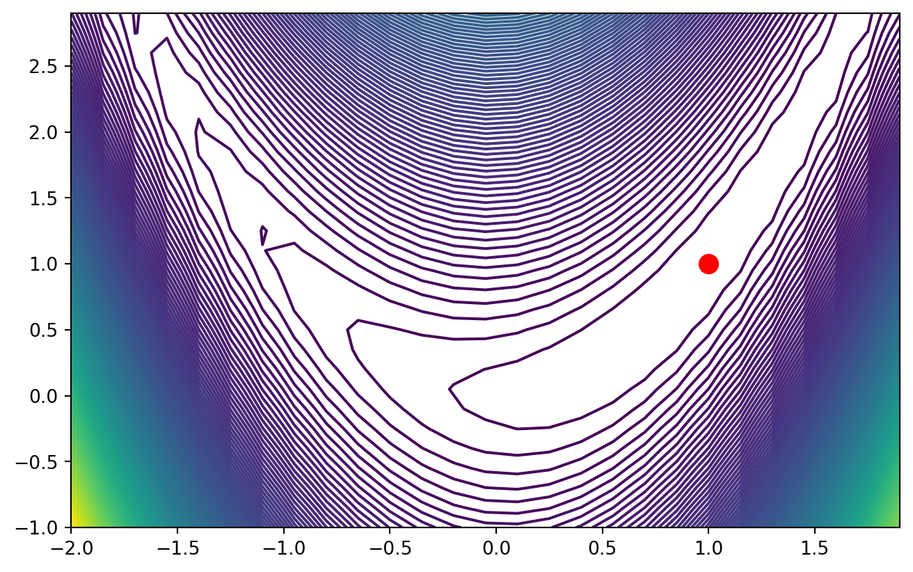
plt.figure(figsize=(8, 5))
plt.contour(X,Y,Z,200)
plt.plot([1],[1],marker='o',markersize=10, color ='r')

Minumum of the Rosenbrock banana function at point (1, 1)

This minumum can be visualized in a contour chart, see figure (banana-min?)

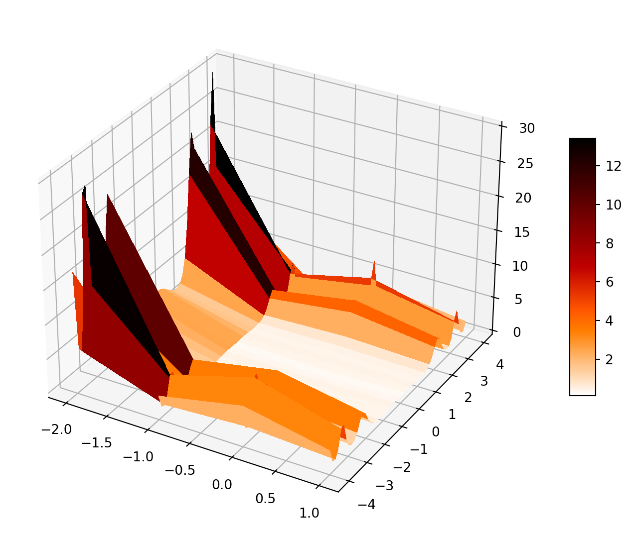
In the last example we uses important information from the objective function; that is, the gradient or first derivatives. Consequently, we can use gradient-based optimization methods such as Newton’s method and conjugate gradient methods to find the minimum of this function. A potential problem arises when we do not know the gradient, or the first derivatives do not exist or are not defined. For example, imagine the following function:

\[f(x, y) = (|x| + |y|)e^{[-\sin(x^2) - \sin(y^2)]}\]

Code

import math
vector = np.vectorize(np.int_)

b = 10
f = lambda x,y: (abs(x) + abs(y))*math.exp((-math.sin(x**2) - math.sin(y**2)))

f2 = np.vectorize(f)

# Initialize figure 
figRos = plt.figure(figsize=(12, 7))
axRos = figRos.add_subplot(projection='3d')

# Evaluate function
X = np.arange(-2, 2, 0.15)
Y = np.arange(-4, 4, 0.15)
X, Y = np.meshgrid(X, Y)
X = vector(X)
Z = f2(X,Y)

# Plot the surface
surf = axRos.plot_surface(X, Y, Z, cmap=cm.gist_heat_r,
                       linewidth=0, antialiased=False)
axRos.set_zlim(0, 30)
figRos.colorbar(surf, shrink=0.5, aspect=10)
plt.show()

The global minimum occurs at \((x, y) = (0,0)\), (module-min?), but the derivatives at \((0,0)\) are not well defined due to the factor \(|x| + |y|\) and there is some discontinuity in the first derivatives. In this case, it is not possible to use gradient-based optimization methods. Obviously, we can use gradient-free method such as the Nelder-Mead downhill simplex method. But as the objective function is multimodal (because of the sine function), such optimization methods are very sensitive to the starting point.

Optimization Sensitive to the Starting Point

If the objective function is multimodal, and the starting point is far from the the sought minimum, the algorithm will usually get stuck in a local minimum and/or simply fail.

Code

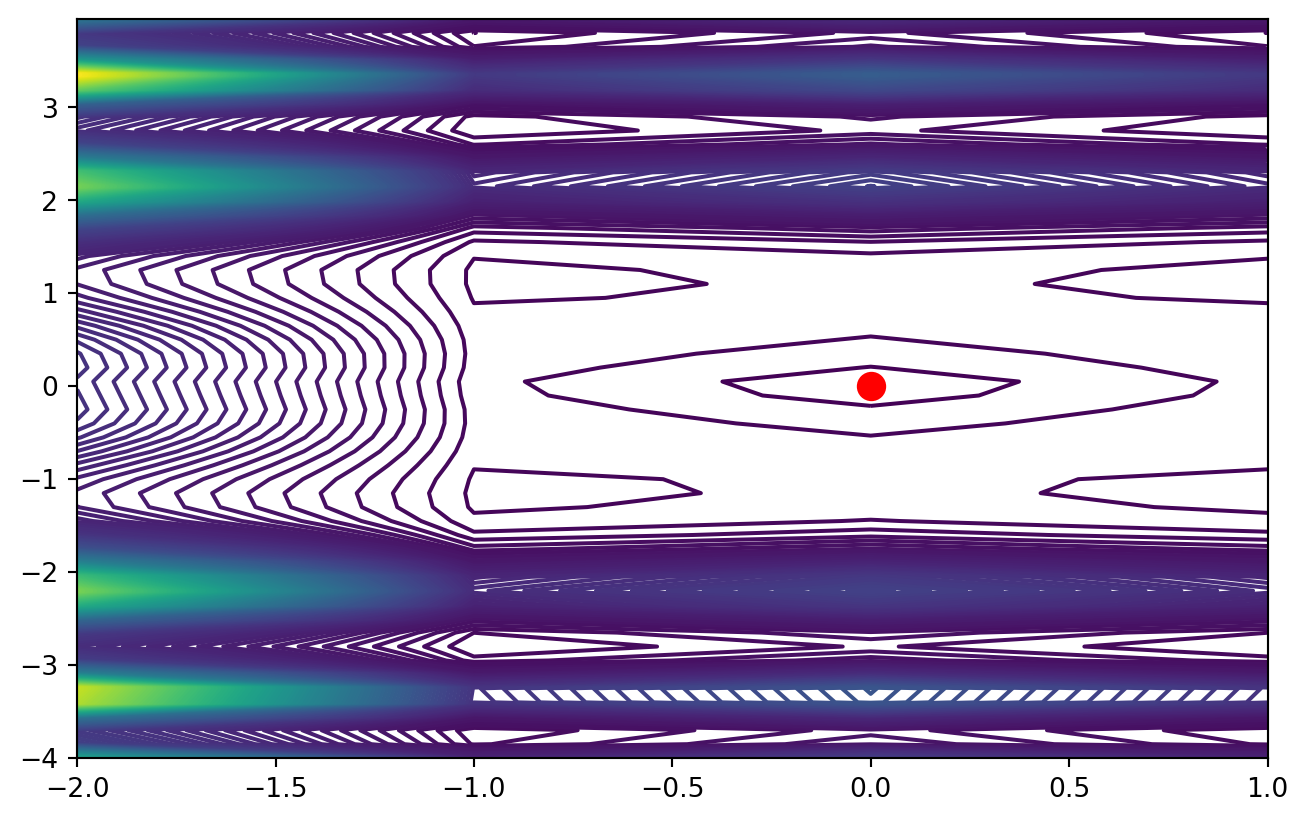
plt.figure(figsize=(8, 5))
plt.contour(X,Y,Z,200)
plt.plot([0],[0],marker='o',markersize=10, color ='r')

Minumum of \(f(x, y) = (|x| + |y|)e^{[-\sin(x^2) - \sin(y^2)]}\) at point (0, 0)

2.1 Integer Programming

2.2 Other topics